

The value of weather data comes from what you do with it. In order to get value from our weather data typically users will import it into other business systems or spreadsheet systems such as Excel or Google Sheets. In this document we will demonstrate how to get a Visual Crossing Weather query directly into Google Sheets as well as make the query dynamically driven by other data on the sheet.
Building the Query
First we will navigate to the following page in our web browser:
https://www.visualcrossing.com/weather-query-builder/
Here we will enter our credentials and begin our query building. If you do not have a login account yet please follow the steps in this document:
How to sign up for a Weather Data Account
This document assumes you know how to build a basic forecast query but if you do not, visit the following document for details:
Getting started with Weather Data Services
To keep it simple, our query is created in only a few clicks. Enter in two locations using the manual options, choose the forecast data option, and retrieve the weather data.
Please make sure the Query you build is a forecast query and choose one or more locations. Once you have completed your query you should see the forecast data for your locations as below. This will be the starting point for our Google Sheets import.
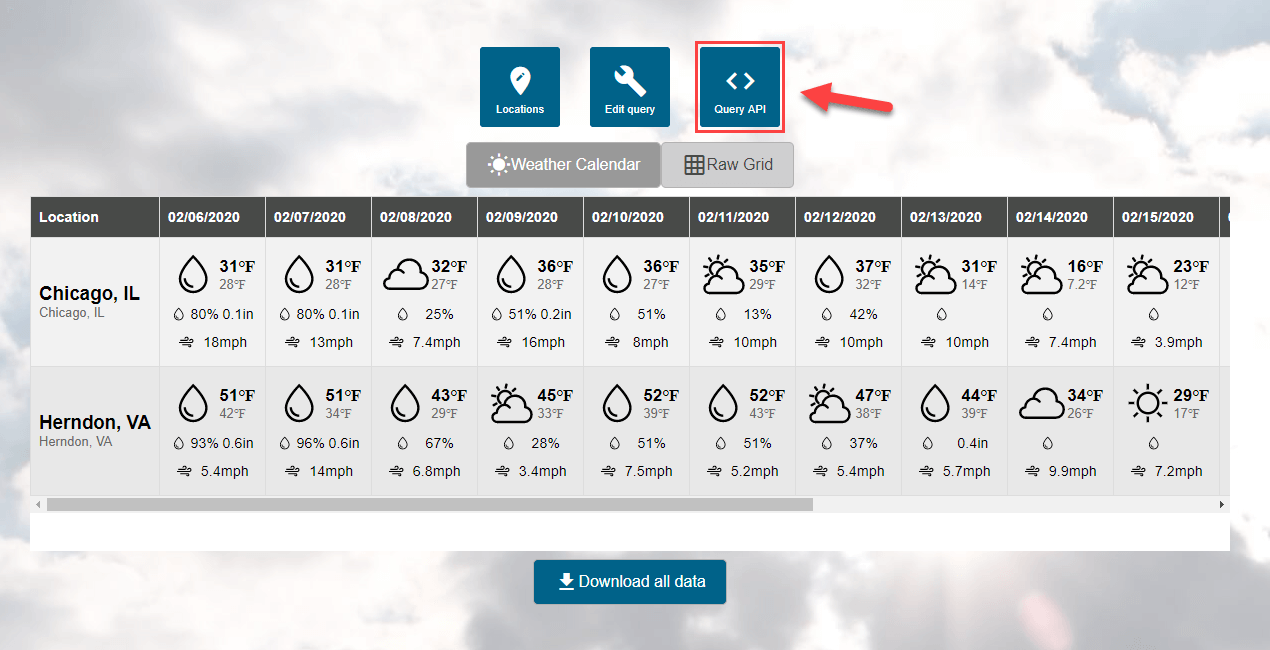
We will begin by selecting the ‘Query API’ button at the top of the data results preview page. This will direct us to the query page where we can capture our URL string.
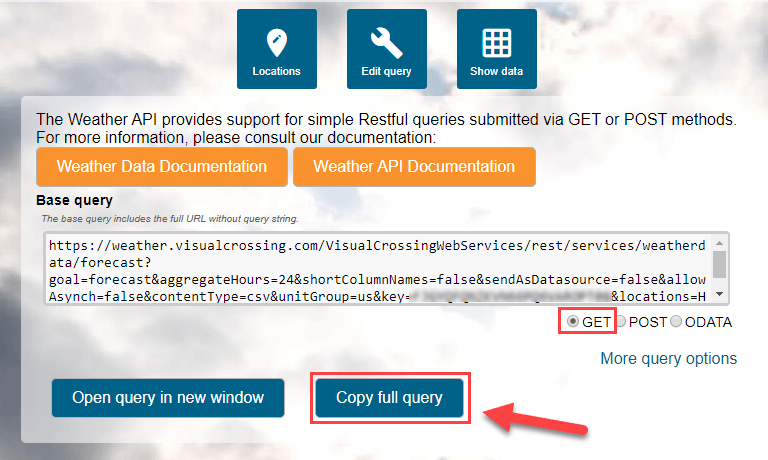
Make sure the query string is of the type ‘GET’ and click on the ‘Copy full query’ button at the bottom. This will copy the entire query string into our system copy-paste buffer. The string that gets copied is the full definition of your query and will allow Google Sheets to fetch the results.
Loading Data in Google Sheets
Visit your Google Sheets account and open a new sheet. On this sheet select a cell about 5-7 rows down the page as seen below.
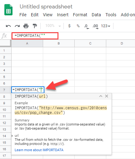
Enter the following text into the cell using your keyboard.
=IMPORTDATA(
As soon as you enter this data the autocomplete system will show you the function ‘IMPORTDATA’ and let us know that it takes exactly one string in quotes as a parameter. It even gives us an example.
This is where we will paste our Weather Query URL that we copied in step one. Making sure that our pasted value is between those quotes. It should look like the following:
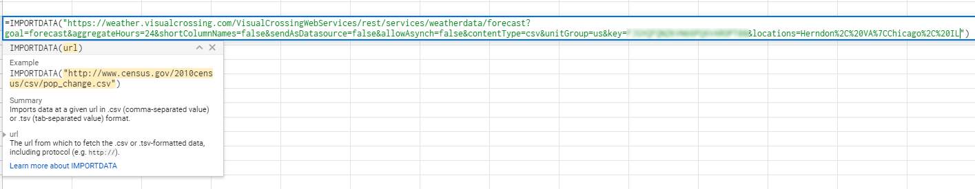
=IMPORTDATA(“https://weather.visualcrossing.com/VisualCrossingWebServices/rest/services/weatherdata/forecast?goal=forecast&aggregateHours=24&shortColumnNames=false&sendAsDatasource=false&allowAsynch=false&contentType=csv&unitGroup=us&key=XXXXXXXXXXXXXXXXXXXXXXXX&locations=Herndon%2C%20VA%7CChicago%2C%20IL”)
Simply by hitting the enter to key to submit the function in the cell you will see confirmation that the query is running.
The system will say “Loading…” until it completes and then we should see our data loaded in, using our cell as the first cell of the new table range it created.

Our first query is complete and now we have weather data in Google Sheets.
Formatting our Data
Some spreadsheet systems have sophisticated data type detection methods but many of them don’t always get the type or formatting the way you like. Typically, date values are the first to require attention. As you can see from out data above the “Date time” column is an integer and not useful for viewing forecast data. Let’s fix that. We will start by selecting the entire column.
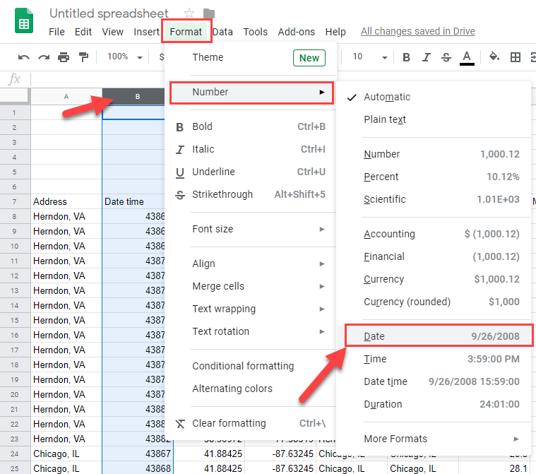
Once we select all of “Column B” which represents our date, we will open the ‘Format’ menu, choose the data type which should say ‘Number’ and then choose the ‘Date’ option which will format our column as a date.
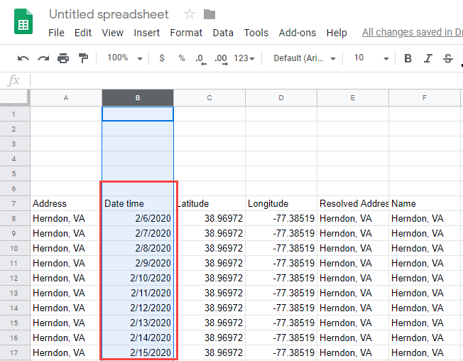
Success! We now have a readable date column for our forecast query dates.
Parameter Driven Queries
What we have loaded is valuable data but if you need to update this data frequently or if you need to change simple parameters such as the location (or dates for historical queries) you will want to drive the query by data found on the spreadsheet. To do this we need have cells as the input to the query and put that inputted data into a format that we can pass in the URL dynamically.
Data Preparation
We will begin by producing a new list of cities we want to query by.
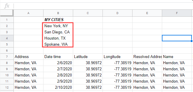
We do this by entering in Location Names as we have done above into empty cells. We have added a column header to our list called “MY CITIES” but this is not part of the data and is not necessary to our task and should not be part of our data range or we will get errors.
Next we will select the area of location names and create a named data range for it to make referencing this area easier. This step is not necessary but makes the implementation cleaner and more foolproof.
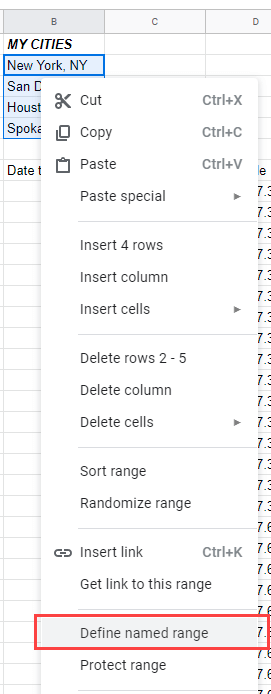
Select our range of location cells and right click to bring up the menu and choose ‘Define named range’.
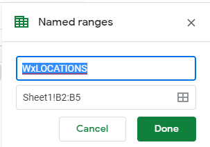
We will name our range “WxLOCATIONS” and click ‘Done’.
Now we that we have our list of locations we must put them in a form that the query can understand. The correct string format for locations in the URL is a pipe (“|”) delimited list. If you looked at the URL you won’t see the pipe symbol or other symbols due to character escaping. The correct format is as follows:
locations=<LOCATION1>|<LOCATION2>| etc…
To create this list we will use the ‘JOIN’ function in Google Sheets and we will construct this in a separate cell just for clarity and demonstration purposes. Start by selecting an empty cell.
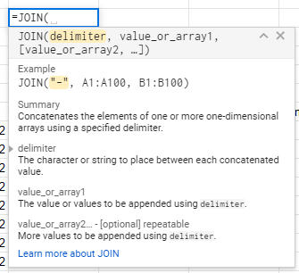
As soon as we type “JOIN(” the system will autocomplete the function and show us the necessary parameters which are first the delimiter and then a list of values. We will enter in “|” to define our delimiter and finish the function with our values by putting in the range name we created above.
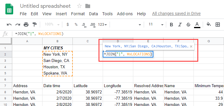
We entered:
=JOIN("|", WxLOCATIONS)
As you can see in the image above Google Sheets will even show a preview of our cell’s value based upon the function and data we gave it. The ‘JOIN’ function correctly walked through the list found at “WxLOCATIONS” and appends them into a single string separated by our pipe delimiter.
Finally, we will create another named range just as we did above for this cell.
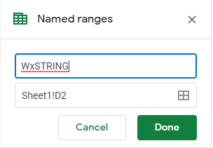
We will name this joined string cell “WxSTRING”. Now in our URL web query we can simply refer to this string to provide the full, pipe-delimited list of weather locations.
Query Modification
We now have a string we can concatenate into our Query String that we originally brought in via the ‘IMPORTDATA’ function. First we need to find the “locations” parameter in our original weather URL.
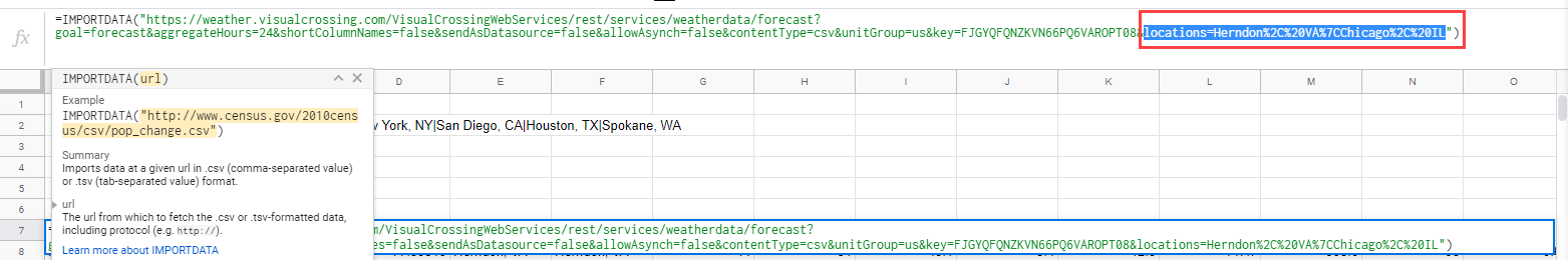
By selecting in the first data table cell we can see the string in the function header and we will remove the following bolded text:
locations=Herndon%2C%20VA%7CChicago%2C%20IL”
and we will end the URL String after the equal sign thus eliminating the hardcoded locations from the original URL. The last part of our new shortened URL will look as follows:
locations=”
This basically ends the URL string at the “locations=” parameter and we will use another function to append our new locations string to the end of this string. We will do this using the ‘CONCATENATE’ function as seen below:
=IMPORTDATA(CONCATENATE(“<Insert Our Shortened URL String Here>”,WxSTRING))
Basically the ‘IMPORTDATA’ function needs a single string and the CONCATENATE function provides that string by combining our newly shortened URL and appending our pipe-delimited list of locations found in “WxSTRING”. The final cell value will look like this:
=IMPORTDATA(CONCATENATE(“https://weather.visualcrossing.com/VisualCrossingWebServices/rest/services/weatherdata/forecast?goal=forecast&aggregateHours=24&shortColumnNames=false&sendAsDatasource=false&allowAsynch=false&contentType=csv&unitGroup=us&key=XXXXXXXXXXXXX&locations=”,WxSTRING))
By simply hitting enter on this cell it will submit the new query and we will see the results of our query that now uses our dynamic list.
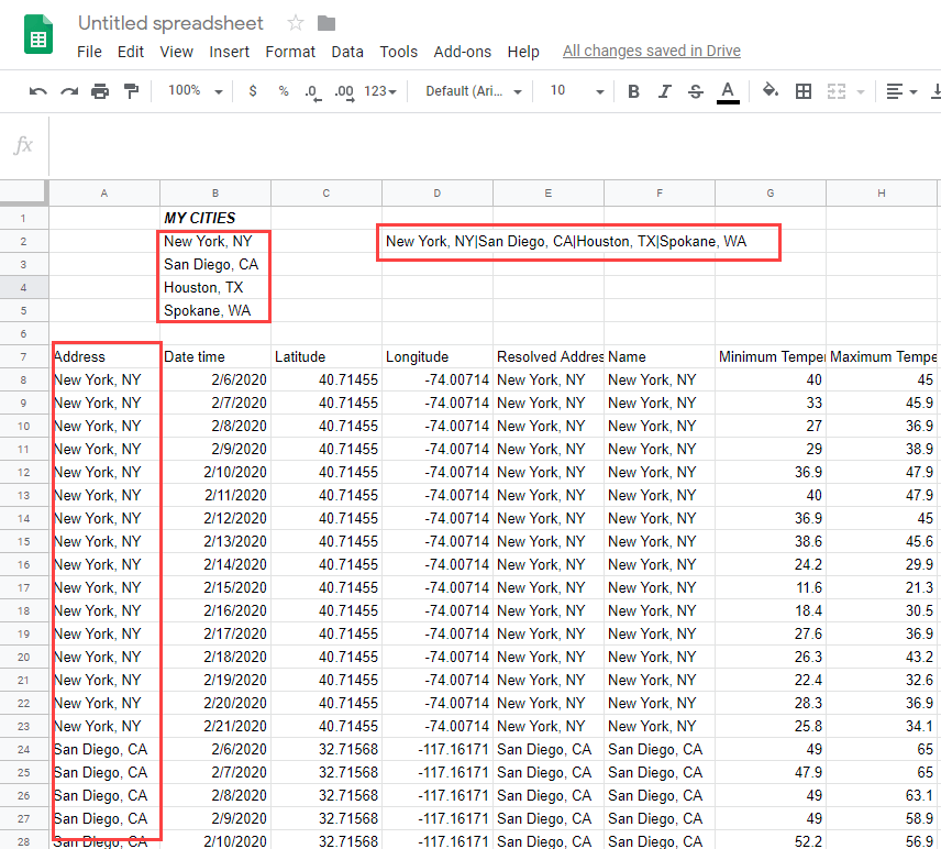
As you can see our query dynamically refreshed itself. You can now simply change cities in our list and the entire spreadsheet will dynamically query the Visual Crossing Weather Data Service for new data every time.
Additional Sources of Information
For more information, interactive discussions please feel free to join our discussions. Also check our our Weather Data FAQ.