

In this article, I’m going to show you how to easily load weather forecast data into your R analysis. We’ll walk through the process step-by-step showing you how to construct the query in Visual Crossing Weather and then use the query URL to import the weather results using R Studio.
If you would like to follow along with a video as well, open a browser on the matching YouTube video here: https://www.youtube.com/watch?v=3puJbAhmnmU
Also see our companion article about importing historical weather data into an R analysis.
The estimated time to complete this exercise is about 5 minutes.
Step 1
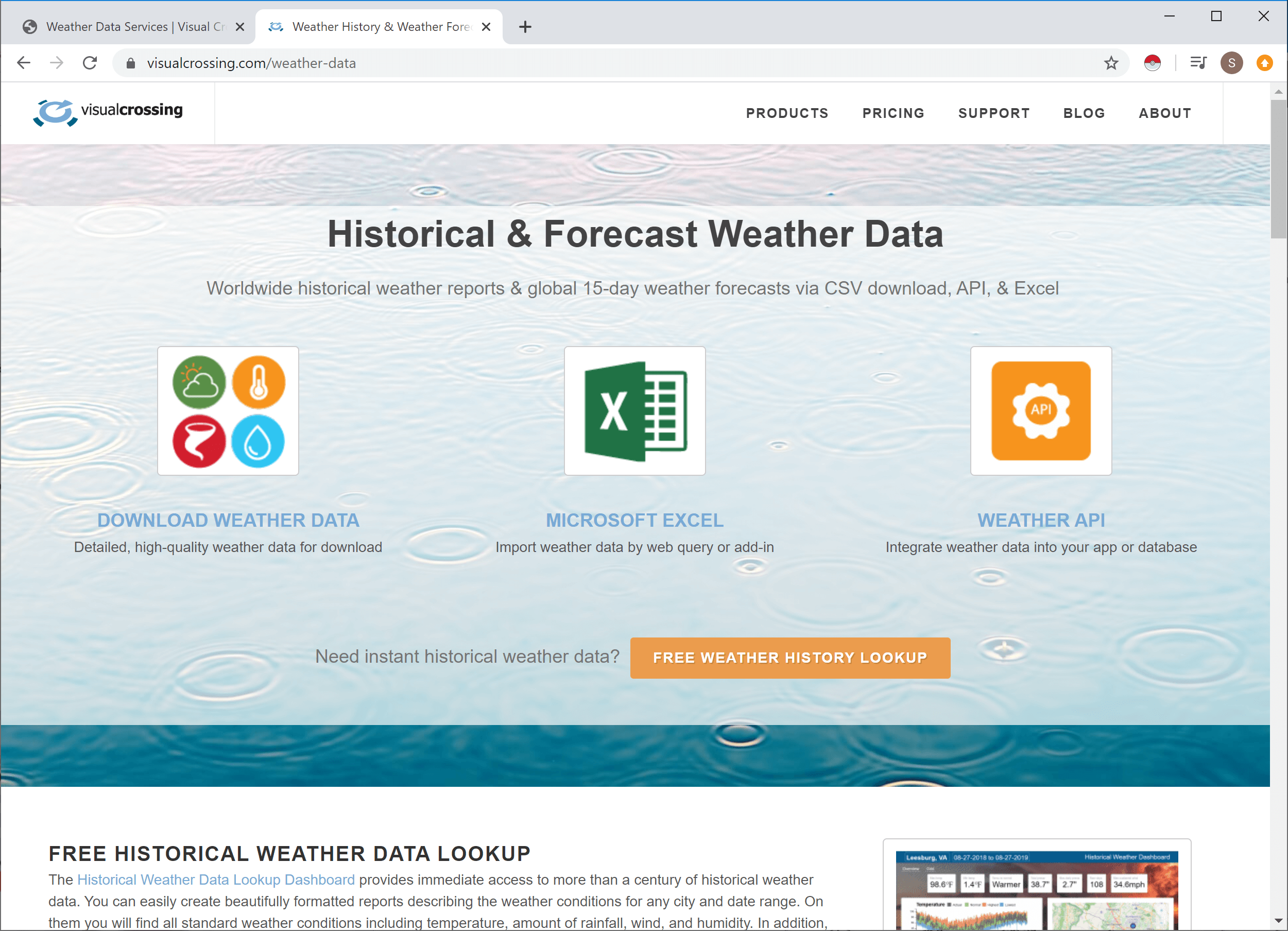
We’ll start by going to the Visual Crossing Weather Data page. We then need to click on the link to go to weather data download page near the top of the page.
Step 2
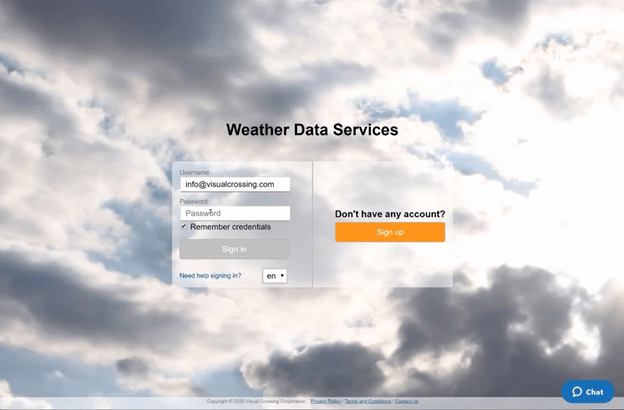
Once on the log-in page, you will need to sign into your Visual Crossing Weather account. If you don’t already have an account simply click on the orange button on the right side of the login page. Signing up for a free trial account will give you immediate access to a full 15-day forecast for any location worldwide.
Step 3
For this example, we’ll select the option to manually enter a location to use for the weather forecast. However, you could instead load a sheet of addresses or paste in a list as plain text if you have those available.
Step 4
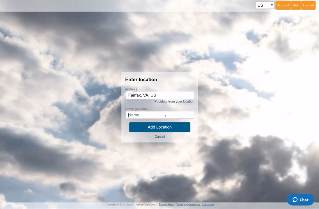
As for the address itself, we’ll tell the system to use our current location by clicking on the “Populate from your location” link below the location text box. However, we could instead manually enter an address, a city name, or a postal code. Optionally, we can also give the location a friendly name for our own reference in the output data. This feature is most useful when you are comparing multiple locations in the same dataset.
Step 5
Next, we need to choose the query type. Since the default option provides a 15-day daily weather forecast, we can simply accept the default for the purpose of this exercise. However, in this panel there are other options as well such as weather history queries, historical data summary reports, and hourly data. These are among the many options covered by our other tutorials and videos. Please take a look at those or reach out to us directly if you need more information on these.
Step 6
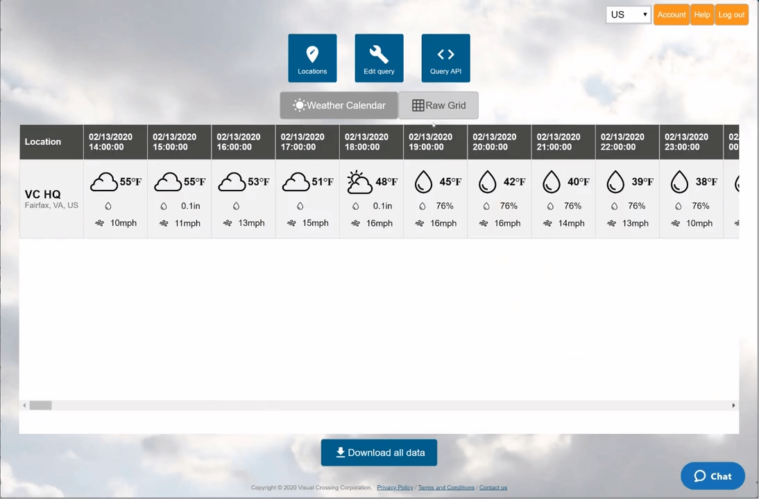
When we run the query the default view is the weather calendar. This view provides a simple overview of the result data. It is extremely useful for comparing data from different locations side-by-side.
Step 7
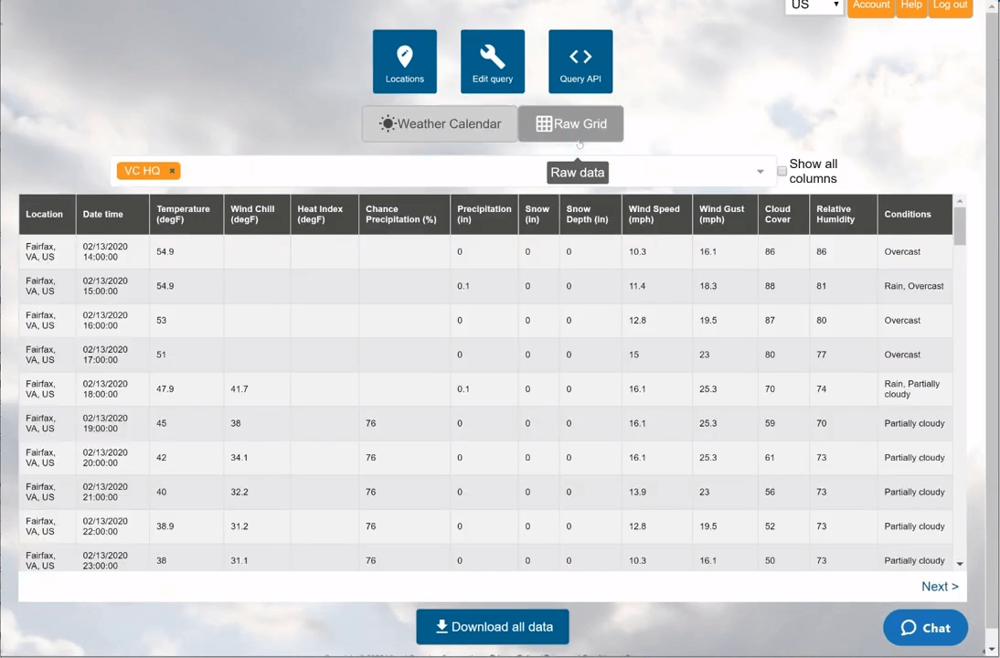
To see more details we can change to the grid view by clicking the “Raw Grid” button near the top of the page. This view gives a single row for each record in the forecast data. In this example, we will have one row of forecast data for each day of the 15-day forecast at the location we selected earlier. You can now see the various weather metrics that are provided in the output data. These include common values such as temperature, precipitation, and wind as well as less common value such as heat index, cloud cover, and wind gusts. For more information on the details and how to use these less common weather metrics, please see our Weather Data Documentation.
Step 8
We could now download the data as a CSV by pressing the “Download all data” button for manual import into various analysis tools, but instead, we’ll switch to the API view to generate the query URL. Using a query URL will allow us to directly import this data into our R code. In addition, this query will allow R to fetch live data and refresh the data as needed. Since the default query URL output is CSV, which R can read directly, we can simply press the “Copy full query” button to copy the query URL to the clipboard.
Step 9
We can now use this URL to load the weather query results directly into R. For this example, we’ll switch to RStudio. Loading the live result data is as simple as entering the URL into R’s read.csv() function. To do so, we would enter a command like the following:
ForecastData <- read.csv(“<URL>”)
Where the “<URL>” is the value the we copied from the Visual Crossing Weather API page.
Step 10
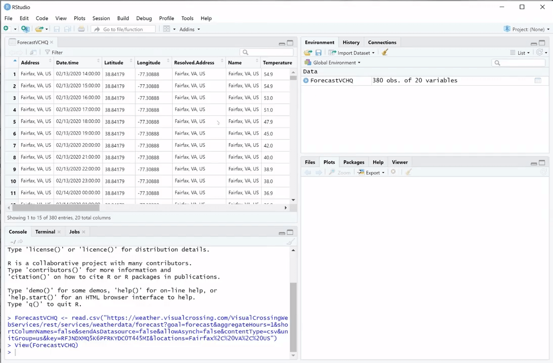
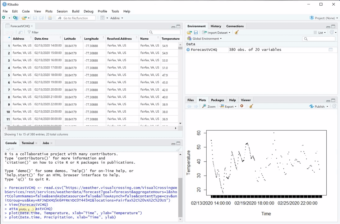
Once loaded, we can view the table in RStudio either by clicking on it or by manually typing the View() command specifying the name of the table that we used above. Now, statistical analysis, plotting, correlating, and reporting, all strengths of R, become easy to apply to all types of weather data queries. In more advanced applications we could adjust the query URL from our code to dynamic change the parameters of the query itself.
If you would like to learn more about using Visual Crossing Weather options such as history data, multiple location import, and use within other analysis tools please see our other tutorials.