

The Visual Crossing Weather Data Service enables users anywhere to load weather data into Excel, Google Sheets, Relational Databases, Business Intelligence Tools and more. We recently released a downloadable Weather Workbook that allows users to query weather data directly into Excel. In this blog we will show you the Multi-Site Forecast Workbook which is a modified variation of the Weather Workbook dedicated to showing the forecast for multiple sites in an Excel Pivot Table for optimal viewing. One of the biggest requests we get from users is the ability have a forecast for just a few weather variables where they can quickly see the forecast for all of their locations in a single view. They also want the capability to easily modify those locations as well as flag any temperatures that are outside of a particular range. Some of these use cases involve construction companies managing work at multiple sites, shipping companies that need to know the forecast to where they are shipping or companies that do site visits and require ideal weather conditions. The Multi-Site Forecast Workbook is a great way to get started and just like Weather Workbook it is 100% modifiable by any of our customers to customize it to their needs.
If you are interested in learning about all the features of the Weather API you can visit the documentation page: Weather API Documentation If you have questions about the weather variables and their definition you can review the following: Weather Data Documentation
Let’s start our tour of the Multi-Site Forecast Workbook.
What is the Multi-Site Forecast Workbook?
The Forecast Workbook is a standard Excel Workbook with defined URL queries to call out to the Visual Crossing Weather Data Service to get weather data forecast and bring it into your workbook. It uses the built-in Excel Power Query feature to execute all data fetches. It also uses the link between the Power Query infrastructure and the Pivot Table features in Excel. The Power Query loads the data from the Visual Crossing server and the Pivot Table nicely pivots the data into a presentable format for us.
How do I get the Multi-Site Forecast Workbook?
This part is simple… Just download it from the following link on the Visual Crossing website:
MULTI-SITE FORECAST WORKBOOK (Using Timeline MultiLocation API)
Other weather workbooks are available on the GitHub: Weather Workbooks on GitHub
Once you save this workbook to your desktop, simply run the Excel Workbook just as you would any other workbook you use. You will also need to have an API Key to send with the query so the server can authenticate your request as being from a registered user. Trial accounts and some paid accounts will provide you with API Key access. To sign up for an account, please follow the steps in this technote.
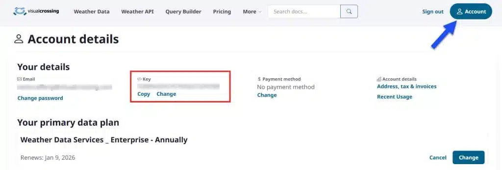
Once you have an account, just click on the “Account” button after signing in and copy the API Key. You will use this below when making your first query.
A Note on Privacy
When you first open the workbook or possibly when you make your first query, the Excel system will warn you that this workbook is making external queries with the data you enter.
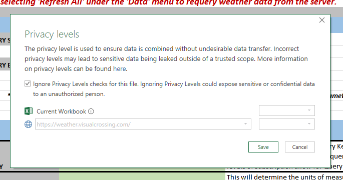
One simple solution is to check the ‘Ignore’ option and continue on. If you are concerned about Privacy or have Corporate policies to adhere to, then please visit the following page on the Microsoft support site to properly set up your Privacy options for Power Query. Also, if you want to know the exact string that is being sent as a query URL, click on the ‘AdminSettings’ sheet of the Forecast Workbook and you can verify all data sent.
Setting Up Your Forecast Workbook
The first step is to open the Forecast Workbook in Excel. Once opened you will find 5 Sheets represented as tabs of your workbook at the bottom of the Excel application:

These tabs are as follows:
Forecast Settings – This is the main user control panel for the workbook. Here you set the locations, set conditions thresholds, enter your API key and monitor alerts for locations.
Daily Forecast Calendar – This is a list of locations in calendar form for the next 15 days. It will show all forecast conditions and color highlight those that are outside of the set values.
Hourly Forecast Calendar – This is similar to the Forecast Calendar but shows hourly data instead of daily aggregations.
RAW DAILY FORECAST DATA (hidden) – This is the raw table of daily forecast result and is only required for debugging purposes.
RAW HOURLY FORECAST DATA (hidden) – This is the raw table of hourly forecast results and is only required for debugging purposes.
Admin Settings (hidden) – This sheet is where the strings that build the query are constructed for submission to the weather server. Only if you are customizing the worksheet should you ever need this page. Technical Support may ask occasionally for you to send them the final query string for debug purposes. the “URLCOPY” sections are particularly useful as you can simply Copy-Paste the cell values into a web browser bar to test the query and get results back.
To make your first query, simply click on the “Forecast Settings” sheet. On this sheet we will see that there are sections colored in green that we need to provide to the worksheet to make our query.
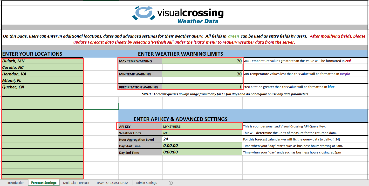
PLEASE NOTE: All user-editable sections in this workbook are color coded with a green background. Let’s get started:
Step 1 – The most important step is to enter in your private API Key into the green box next to the “API KEY” label.
Step 2 – In the ‘ENTER YOUR LOCATIONS’ section at the left, enter a few locations that you wish to query on. These can be addresses, cities, zip codes, etc…
Step 3 – Finally, we can set our threshold warning levels. These are values that will search the table’s Temperature and Precipitation Values and color code those that fall out of the standard range. You can set these values as you wish and will apply to any value regardless of which standard measures type you are choosing. It simply compares values and highlights those values as needed.
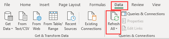
FINAL STEP – Now that we have our Forecast Query defined, we can fetch the data simply by using the ‘Refresh’ functionality of the Excel Power Query system. To do this, click on the ‘Data’ menu and click on “Refresh All”.
This action will refresh every query in the workbook. Below, we describe other options you have for submitting/refreshing queries. We can now click over to either our RAW FORECAST DATA or Multi-Site Forecast sheets and see the results of our query with the locations we requested.
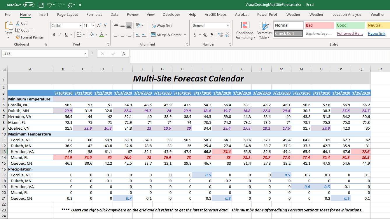
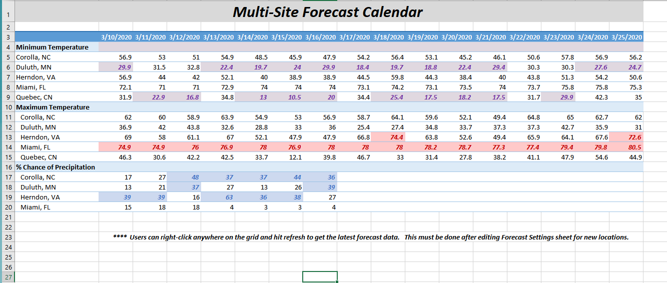
You can now see that the Multi-Site Forecast Calendar has fetched the latest forecast for all of your locations, but it has also highlighted values that have exceptional conditions as set by you. You may have noticed that we have chosen only 3 weather variables as these are the most popular for users to track. However, below in this document you can customize this view with just a few clicks and show additional weather variables.
Refreshing Data
One of the first questions users have is about the need to click on “Refresh All” to update the data. Users can simply right-click on the datasets and refresh Forecast independently. There are many other refresh options here that you can choose to add and those are defined in How to automatically refresh Weather Data in Microsoft Excel.
There are many good options and if you need help just contact support
How do I Customize or Integrate this into my Workbooks?
Just as with Weather Workbook, the Forecast Workbook is fully yours to edit and copy as you need. This is a service we provide to our customers to use as a weather data download tool, query builder or as a starting point for a custom workbook designed for specific users. Most users will start by simply copying or adding their own sheets that can refer to the weather data being fetched. If you wish to move around the data entry cells onto another page or to co-exist with the date that is retrieved, you can simply Cut and Paste the data entry cells to another place in your workbook. NOTE: YOU MUST MAKE CERTAIN THAT THE NAMED RANGE OF THE ENTRY CELL REMAINS INTACT ON PASTE. If the name is the same, it will be pasted into the URL Query just as before. For example, if you want to move the Locations List you can select the entire green section (note the name of this section) and simply cut and paste elsewhere in the workbook.
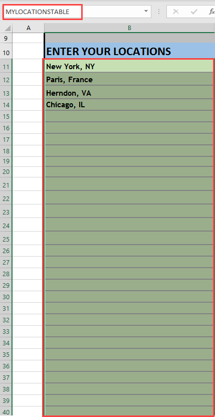
Just remember that the URLs are constructed by referencing these fixed named areas so they must exist and be populated somewhere in the workbook. To see the name of the entry cell, just click on it and see the defined name as we did above.
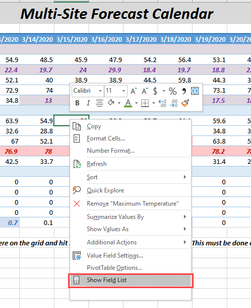
Another common customization is the ability change or limit the variables. As previously stated, we started with Max Temperature, Min Temperature and Precipitation. However, since we are using a Pivot Table the user can create any Forecast Calendar View they wish. Here is how… On the ‘Multi-Site Forecast’ Sheet, right-click anywhere on the grid of data and choose to ‘Show Field List’:
This action will enable the Excel’s Pivot Table editor to open up which allows you to design the table. We recommend starting simple as we will do here. Instead of changing the structure we are simply going to turn off and on new weather variables.
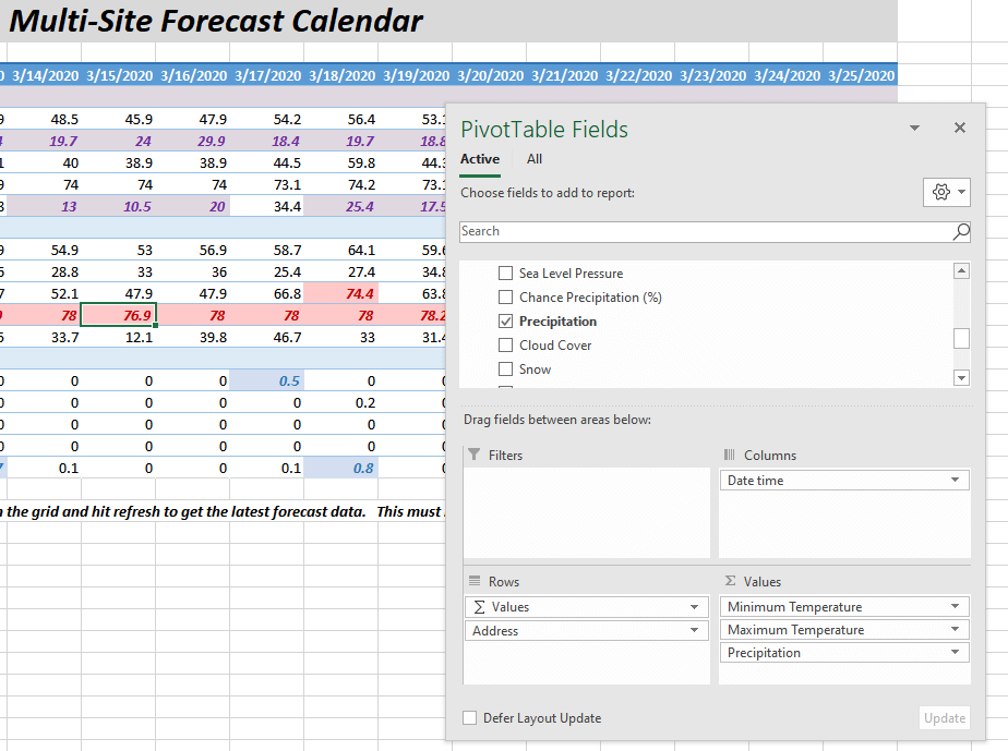
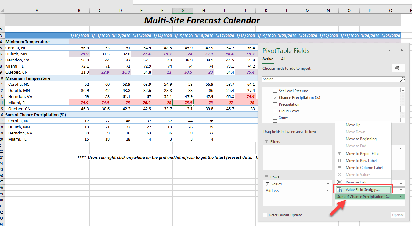
With the Pivot Table Fields window open, uncheck “Precipitation” which will turn off that variable from the view and check “Chance of Precipitation”. Notice below that the table updates appropriately. But also notice that the name for our new weather variable is not correct and the aggregation value is not correct. Click on the “Sum of Chance of Precipitation” as seen below and choose “Value Field Settings”.
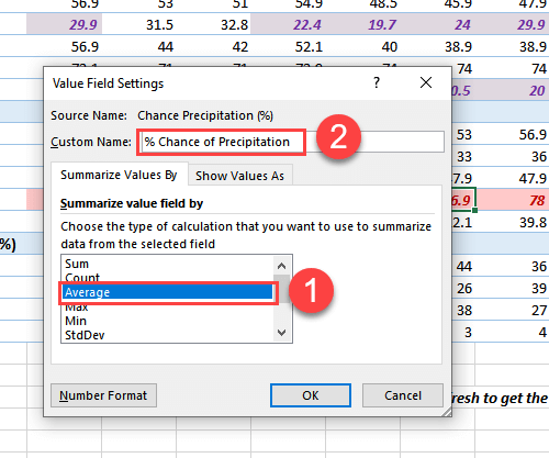
This editor will allow us to rename the new weather variable and change its aggregation. Start by choosing ‘Avg’ as the aggregation type and then change the name to “% Chance of Precipitation”.
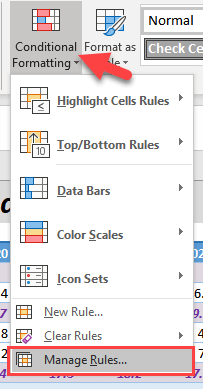
You can now see that the data is updated with your new variable. However the colored threshold was for the previous variable. We can simply reuse the older one and rename the field. To do this we can select a field of the new variable and click on the ‘Conditional Formatting’ button on the Ribbon Bar. And choose to ‘Manage Rules’.
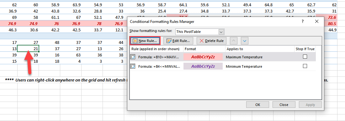
Now we can see that our 3rd rule regarding precipitation is gone but our temperature rules still exist. To recreate one, simply select “New Rule”. Please note that we must know at least one cell in our new range of data to define a rule. We clicked in ours as seen below to highlight it.
After selecting new rule, we can define ours:
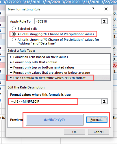
By choosing “All cells showing % Chance of Precipitation” we are telling the system to apply this rule to all values for this weather variable, not just the one cell. Next we choose to use a formula which allows us to the use the Forecast Setting cells to let the user the set the threshold, then we define the formula as being “equal to any cell in our range greater or equal to the value found in the MINPRECIP setting. (labeled as “PRECIPITATION WARNING”)
For us it is shown as:
=c18>=MINPRECIPNOTE: We use cell c18 but yours can be any cell value in range for this weather variable. Our settings above will apply this rule to all values for this variable. Finally, define the colors for the font and background you would like to see and you are done. Click OK. By setting our “PRECIPITATION WARNING” value on the ‘Forecast Settings’ page to 30 (meaning 30% chance of rain) then you should similar to the following:
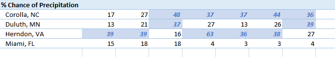
We have now completed our customization and have a new weather variable to monitor for our locations.
Questions or need help?
If you have a question or need help, please post on our actively monitored forum for the fastest replies. You can also contact our Support Team.